
My experience in control robots
from standard methods

Hello, everyone, I'd like to thank the reviewers for attending my presentation, albeit electronically.
I am Gastone Pietro Rosati Papini a post doc researcher at the University of Trento,
and today I will introduce you "Modeling and control of intelligent robots from standard methods to adaptive physical and bio inspired data driven approaches" through my career
Today the use of robotics is coming out of the factories this is opening up new interesting challenges.
Here some examples as:
- Dealing with human or uncertain environment
- Guarantee of safety
- Dealing with failures or partial and uncertain measure
- And others that are listed on the slide
Let's consider the standard approaches, what is the most relevant limitation?
That it is difficult to model everything moreover in presence of uncertainties.
But the behaviour of mechanical systems is well known, it is predictable and we can guarantee its stability and safety.
Whereas on the other hand we have data-driven approaches.
These approaches are very flexible and modular but in robotics it is difficult and dangerous to collect data because it's necessary a machine that interacts with humans or the environment.
And as we know these approaches need of huge amount of data for working.
Moreover the classic network are black-box so it is difficult to guaranty safety.
But in robotics we have a lot of models that we didn't have for image recognition.
So, how can the two approaches be combined?
The idea is to use physical and biological inspiration to structure the neural network and guide the process of learning, and in this presentation I will introduce some preliminary results in this way.
University
Bachelor's Degree
Software Engineering
- Programming languages
- Software skill
- Realtime systems
- Networking devices
Master's Degree
Automation engineering
- Mechatronics system
- Mechanic modelling
- Control theory
- Robotics


:(){ :|:& };:
In this slide I just wanted to show my multidisciplinary background particularly suitable for the type of project I want to realize.
The pictures show some projects I accomplished during my carrier, in both bachelor and master university.
The bachelor more suitable for data-driven approach, and master focused on mechanics and control theory.
This was my master thesis, the goal was to make a robust controller for the arm of the body extender system a fullbody machine realized at Percro Laboratory of Scuola Superiore Sant'Anna.
The video shows, the system in action, I was driving the arm using an internal force sensor, perceiving the robotic arm as a mass in the vacuum.
Let see the controller.
Control System - on single joint
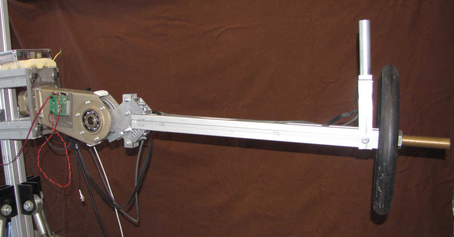

The objective was to control the upper limb of the Body Extender using a force sensor, between the user and the extender.
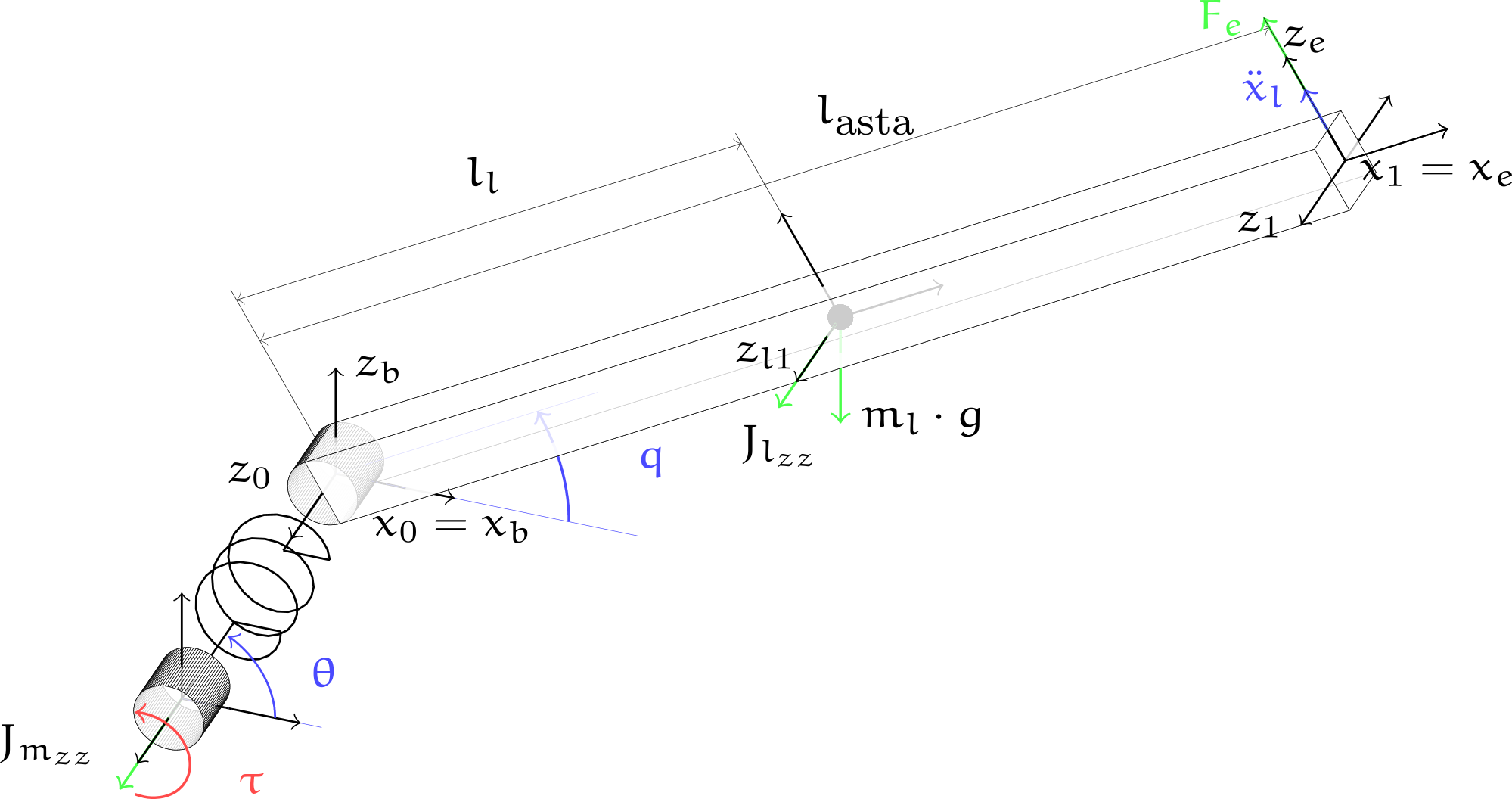
As a preliminary work I focused on a single degree of freedom joint, that I modelled, shown on the left of the slide.
The aim of the control law, it is to make the user perceives a percentage of the weight and inertia of the lifted load, while when the system is unloaded perceive a virtual inertia.
The trajectory is generated by admittance control and followed using a feedback linearization.
Since there was no sensor to the outside, it was necessary to develop an estimator that evaluated the parameters in terms of masses and inertia of the lifted load.
I want to focus on this component.
Results - Testing of the system

The video shows the system in operation during loading and unloading of a 20 kg weight.
The monitor shows the parameters estimation and position tracking, while I perform free movements, controlling the joint using a force sensor.
On the left is shown the relation between the acceleration of the arm against the force measured by the sensor.
The behavior of the system is linear as expected for different load carried, that are: free motion, 10 kg, and 20 kg.
The slope of regression lines represents the value of virtual inertia, here 1.5kg, while the value of the force sensor for null acceleration indicates the virtual mass perceived, one-tenth, of the real mass.
Model based approach - Explicit self tuning control
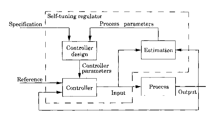
The control system is an adaptive controller defined as:
- explicit self tuning control
The regulator is updated through the system parameters.
In our case the characteristics are:
- The controller is model based
- Parameter estimator (estimation) is model based
— Åström, Karl J. and Wittenmark, B. Adaptive control. Courier Corporation, 2013.
This was an example of adaptive model based control in particular the schema is called explicit self tuning control.
In this schema the regulator is updated through the system parameters.
In my implementation both controller and parameter estimator were model-based.
This is a first example of adaptive behavior that go toward a data-driven approach.
Let's get on with my PhD research
PhD - Main Activities
- Veritas (FP7-ICT 247765) - European project focused on empathic design
A desktop haptic device is employed to induce a programmable hand-tremor on healthy subjects
The main activities I want to illustrate are Veritas:
European project focused on empathic design. The empathic design consists in giving, in particular to the designer, tools to feel at first hand the sensations of an ill subject.
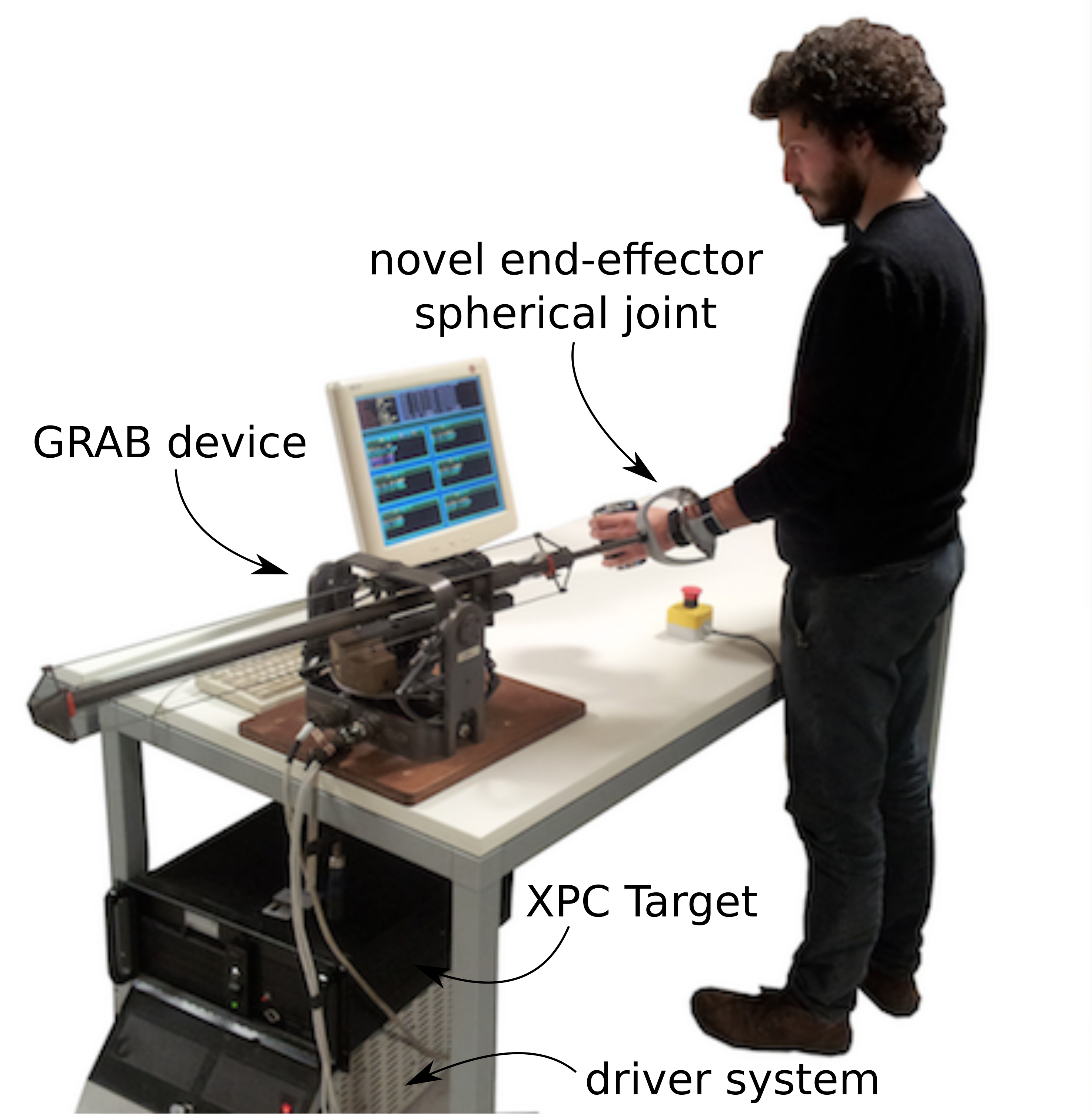
The project was focused on the developing of a desktop haptic device to induce a programmable hand-tremor on healthy subjects that is typically observed in people affected by some kind of neurological diseases
The second project I want to show you is Polywec, which I did my phd thesis on.
Polywec is a project focused on how to convert marine wave energy exploiting electro-active polymers as a variable capacitor.
Veritas Project - Desktop haptic interface for hand tremor induction
Parkinsonian user

— Rosati Papini, G.P. et al."Haptic hand-tremor simulation for enhancing empathy with disabled users." 2013 IEEE RO-MAN.
— Rosati Papini, G.P. et al."Desktop haptic interface for simulation of hand-tremor." IEEE Transactions on Haptics, 2015.
Let's start with veritas, in this project:
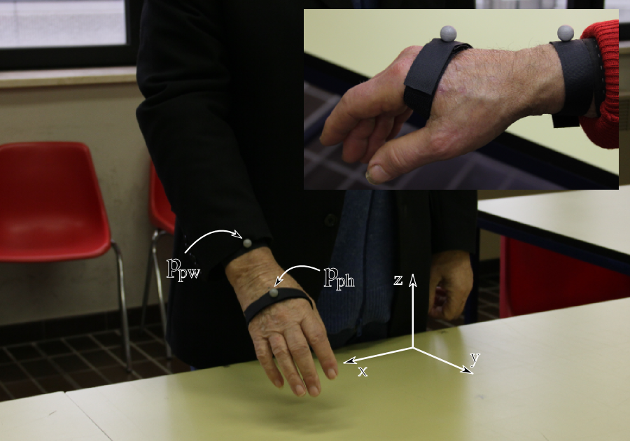
I conducted a campaign for recording wrist and hand vibration of parkinson affected subjects. A picture of the camping is shown in top left of the slide.
I modeled the haptic device, shown in the bottom left. The video shows a preliminary test performed by myself through a graphic tablet that evaluates the type of tremor analyzing how the user makes a spiral.
The spiral is one of the typical test that is used to evaluated the hand-tremor.
To get this results I devèloped an adaptive controller that would induce the recorded vibration on a healthy subject while keeping the subject free to move.
The recorded signal is used as reference trajectory in open loop, while to compensate the amplitude error is used the human impedance estimator. Also here I want to emphasize the adaptive component.

Human impedance estimator
Why is needed?
- Because the system is used by different person

- RMS amplitude with time window of 1 sec: \(E(s)\)
- Filtered wrist reference position: \(x_{pw}^*\)
- Filtered wrist position: \(\widehat{x}_{uw}^*\)
- Human impedance estimator is a PID regulator: \(M_e(s)\)
- Estimated human impedance: \(\hat{m}_{h}\)
System compensator
Position estimator
The adaptive component is needed because many different users can use the device.
The adaptive component of the system is realized by a PID regulator based on the amplitude error between the recorded signal and the measured one, Me.
The amplitude is calculated as RMS amplitude with a time window of 1 second, E of s.
The estimated impedance enters into the system compensator and the position estimator to adjust their behavior.
Results - Testing of the device
Designer of Indesit company testing our device on a gas hob


— Rosati Papini, G.P. et al."Desktop haptic interface for simulation of hand-tremor." IEEE Transactions on Haptics, 2015.
The video shows the use of our device by an Indesit designer.
Thanks to our system he was able to feel the discomfort that people with parkinson's disease have when using the hob and then try to redesign the system.
One result of this process was for example a new stove handle easier to use.
Model based approach - Model reference adaptive control
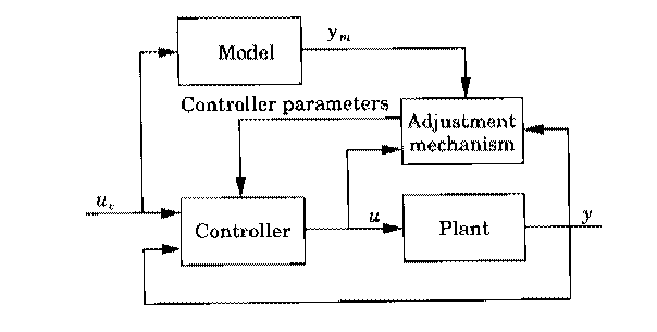
The control system is an adaptive controller defined as:
- Model reference adaptive systems
The adjustment mechanism set the controller parameters in such a way that the error between \(y\) and \(y_m\) is small.
In our case the characteristics are:
- the controller is model based
- reference amplitude estimator (model reference) is not based on physical model
- mass estimator (adjustment mechanism) is not based on physical model
— Åström, Karl J. and Wittenmark, B. Adaptive control. Courier Corporation, 2013.
Again, I investigated the use of an adaptive controller because a standard controller was not sufficient.
The schema is called model reference adaptive system.
The adjustment mechanism set the controller parameters in such a way to reduce error between reference signal and measured one.
Here the controller is model based, whereas the estimator is not based on physical model, because it is just a PID regulator.
PolyWec Project - Exploiting electroactive polymers for wave energy conversion

- Preliminary studies on the energy production of Poly-OWC
Compiled simulink schema for the energy production evaluation - Hardware in the loop tests
Testing different control schemas and harvesting cycles - Experimental tests
Implementation of control schema and video analisys for energy harvesting evaluation - Optimal control for Poly-OWC
Real-time controller for maximizing the energy estration of the Poly-OWC
Let's switch to Polywec. Polywec was a long project in which I made contributions in various forms.
I studied the energy production of Poly-OWC, realizing compiled simulink schema.
I tested different control schemas and harvesting cycles using a Hardware in the loop system.
I partecipated to many different test campaing and I developed a video analisys software for energy harvesting evaluation.
I synthesized a real time controller that maximize the energy extration from the poly-OWC using the results obtained from an optimization procedure.
On this last topic I wrote my PHD thesis, and I want to show you in detail.
Control of an OWC wave energy converter based on DEG


In order to devèlop an optimization procedure to determine which is the best electric field profile to apply on the electroactive polymer for maximizing the energy produced by the PolyOWC system:
I modeled the oscillating water column system.
I modeled the inflatable circular diaphragm dielectric elastomer generator that is on the top of the OWC chamber, an it inflates when the level of water inside the chamber increase.
The model is based on the force tip equilibrium between the differential pressure and the stresses.
The model of the membrane is coupled with adiabatic transformation to generate the constrains for the optimization procedure.
The two curves fmin and fmax represents the force that the mambrain can generete depending on the inner water level and electric field applied on it.
The optimization procedure starts from the definition of the objective function:
that is to maximize the extracted energy within a period.
The energy extrated is written as the product between the fpto (that is the force applied from the membrane to the water) and the velocity of the inner witer level nu.
To perform the optimization I need to write the objective function using only one variable.
Starting from the cummin's equation that represents the oscillating water column dynamics, I writed the state space, I discretized and determined the evolution within a period of the inner water level as function of the fpto and
fe.
where fe is the exitation force.
The constrints are defined by the operation limits fmin and fmax of the membrane as exaplain before.
So I can perform the optimization procudure.
Results - Optimal Cycles

— Rosati Papini, G.P. et al. "Control of an OWC wave energy converter based on DEG." Nonlinear Dynamics, 2018.
An example of the result is shown here.
The two pictures show the optimal electric field profile for two different sea states, but this behaviour is repitable for all sea states.
With yellow is represented the electric field applied on the membrane, that is our control variable, while in black the elevation of the membrane tip.
The charging is realized when the membrane is most deformed, but the instant of charging depends to the frequency and amplitude of incoming wave.
This behaviour has the following explanation.
Because the electric field decrese the stiffness of the mambrane, more time it is kept activated less it is stiff.
So the membrane is kept activated for more time when the period of the incoming wave is longer and less when is shorter.
From optimal control to a real-time controller for Poly-OWC

- From direct inspection of the results of the optimal control is obtained real-time controller
- Lookup table defines the optimal time to charge using \(\dot{p}_{th}\) based on \(H_s,T_e\)
As explained before, given the repeatability of the optimal charging cycles it was possible to synthesize a heuristic that could work in real-time.
This heuristic consists in charging the membrain when the capacitance close to maximum and discharge when is minimum.
This heuristic uses a lookup table to define the best charging instant using a threshold on the derivative of the pressure based on incoming wave parameters.
In this slide is shown the system in actions.
Model based approach - Gain scheduling controller
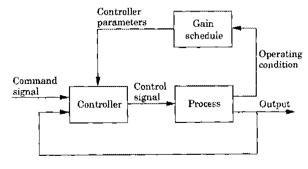
The control system is an adaptive controller defined as:
- gain scheduling controller
the gain schedule adjusts the controller parameters on the basis of the operating conditions.
In out case the characteristics are:
- the control logic is derived from optimal control solutions
- the lookup table (gain schedule) is based on incoming wave parameters
— Åström, Karl J. and Wittenmark, B. Adaptive control. Courier Corporation, 2013.
Also in this case I used an adaptive control schema called gain scheduling controller.
Referring to the picture in our case the controller is derived from optimal control solutions and gain schedule, is based on the incoming wave parameters that are the operating condition.
Now I present the first preliminary results obtained during my PostDoc at the University of Trento, focusing on the objective of the presentation.
What have we seen so far?
Applications of stadard methods from adaptive controller to optimal control.
But can we be more flexible and adaptive? The answer is Yes.
Mixing the flexibility of the data driven methods.
Obtaining neural network with physical structure and reinforcement learning on high level behaviors.
So I want to present the first preliminary results obtained in the Dreams4Cars project.
Dreams4Cars (H2020 731593)- bio-inspired artificial autonomous agent
The cognitive architecture is applied to autonomous driving
- The agent use the motor cortex concept, that is a control space
- Each point in the motor cortex is an action encodes a minimum jerk trajectory
- The points are weighted using the action biasing
- The best trajectory is choosen using action selection
- Then it is converted to control signal by inverse models
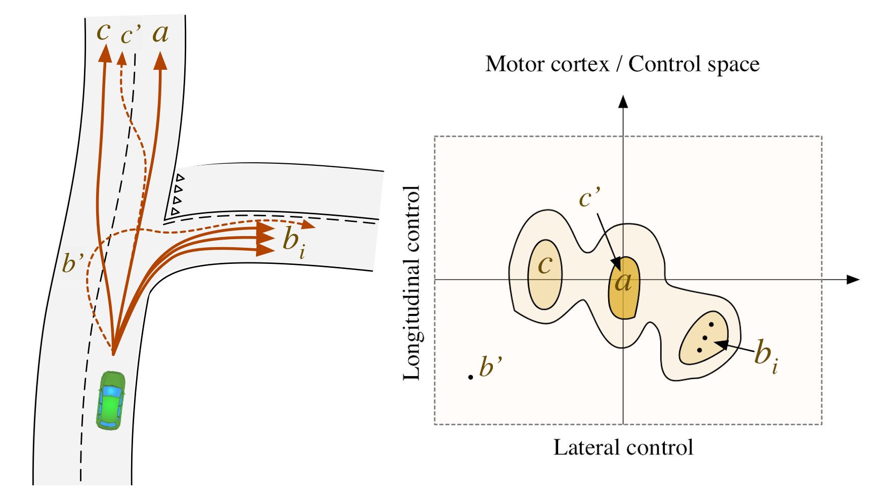
— Da Lio, M., Riccardo, D. and Rosati Papini, G.P. "Agent Architecture for Adaptive Behaviours in Autonomous Driving", IEEE Access, 2020.
Dreams4Cars is a robotics project that sees the development of a bio-inspired autonomous agent. The cognitive architecture is applied to autonomous driving.
- The bio-inspired agent uses the motor cortex concept that is a way to represent the control space.
- Each point in the motor cortex is an action encodes a minimum jerk trajectory (red arrow in the brain).
- The points are biased to steer the system (yellow arrow) for example to implement traffic rules, then
- The best trajectory is choosen using action selection (green arrow)
- From best trajectory we use a inverse model, instead of the classic MPC, to get the steering wheel and accelerator controls for vehicle (blue and purple arrow)
Dreams4Cars - Activities
Each activity covers a different branch of the cognitive architecture
-
Stability and robustness analisys of vehicle lateral control based on dynamics quasi-cancellation:
- Action priming → Action selection → Motor output
-
Robust decision making based on multi-hypothesis sequential probability ratio test:
- Action selection
\( \begin{array}{l} \hline \text { MSPRT algorithm } \\ \hline \text{ Result: Action log-likelihood } \\ \mathcal{M}_{\text {list }} \leftarrow \mathcal{M}_{t} ; (\text{with}~\mathcal{M}~\text{motor cortex}) \\ \overline{\mathcal{M}} \leftarrow \text{mean}\left(\mathcal{M}_{\text{list}}\right);\\ \text{compute likelihood: } L(t) = \overline{\mathcal{M}}-\log \sum_{k=1}^{N} \exp \left(\overline{\mathcal{M}}_{k}\right) \\ \text { if } \max (\exp (L))>\text { threshold then } \\ \quad \left| \begin{array}{l}\text{ take}~\text{action}~\text{with}~\text{higher}~\text{evidence};\\~\mathcal{M}_{\text {list }}=\lambda \overline{\mathcal{M}}; \end{array} \right. \\ \text { else } \\ \quad \left| \text { follow previous action; } \right. \\ \text { end } \end{array} \) -
Flexible modelling of vehicle dynamics with neural networks:
- Simulation and Motor outuput
-
Deal with uncertainties via reinforcement lerning:
- Simulation for Action biasing
In this framework I participated in several works that cover different components of the architecture shown. In particular:
- Stability and robustness analisys of vehicle lateral control based on dynamics quasi-cancellation. A work aimed at analyzing the stability of the control loop when the model is not exactly canceled by the inverse control.
- Robust way to perform action selection within the control space.
- Flexible and modular approach for modelling longitudinal vehicle dynamics, that is the first topic that I want to exaplain in details
- and how to deal with uncertain situation via reinforcement lerning, that is the second
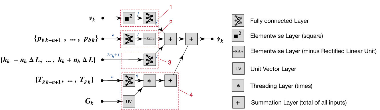
Modelling longitudinal vehicle dynamics with neural networks
Causal system

\( \definecolor{myRed}{RGB}{234,26,8} \definecolor{myGreen}{RGB}{50,153,5} \definecolor{myBlue}{RGB}{0,10,206} \definecolor{myYellow}{RGB}{205,255,3} \begin{aligned} {\color{myYellow}a} &= \frac{1}{M} \sum_{i=1}^{m} F_{i} \\ &= {\color{myRed}F_\text{b}}+{\color{myGreen}F_e
g_r} + {\color{myBlue}F_a} + {\color{white}F_s} \end{aligned}\)
In this work we started from the assumption that the vehicle is a causal system and the forces acting on it can be considered additive.
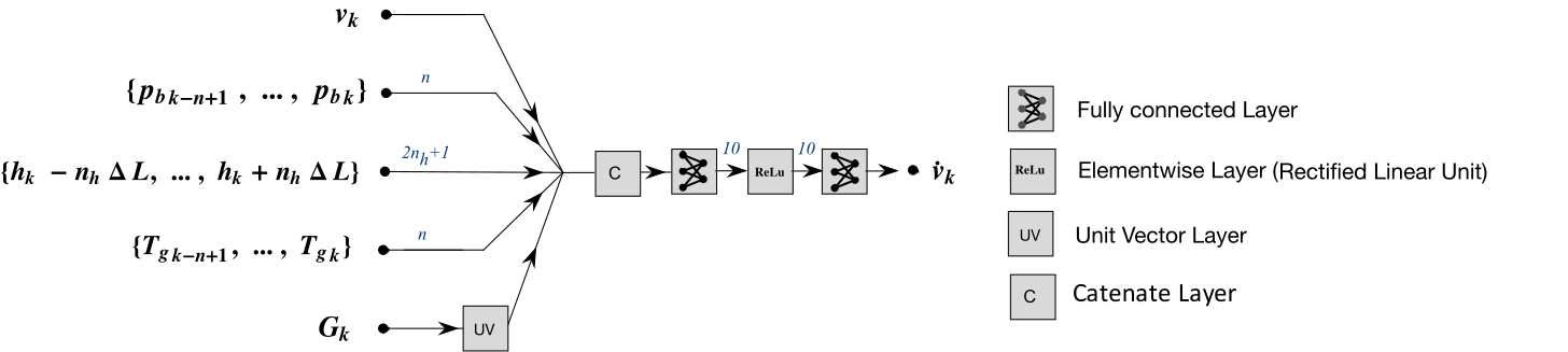
In the picture is depicted the neural network. Here the structure the novel element. Each branch of the network represent a force contribute:
- The air drag in blue.
- The slope of the road in white and black.
- The engine with the relative grear in green.
- The brake in red.
- The output of the network is the predicted accelleration in yellow.
Network models for longitudinal vehicle dynamics
Neural networks with inspired physical structure
Convolutional
Recurrent
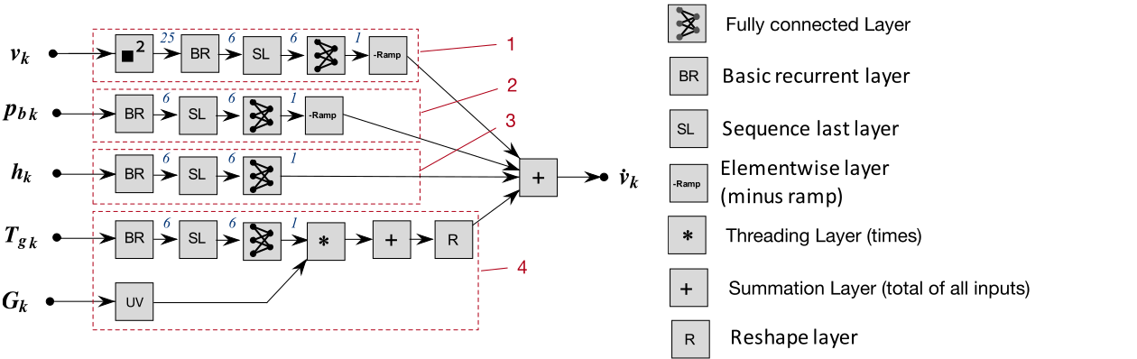
Unstructured networks
Convolutional
Recurrent
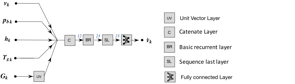
Here are the other structures we analyzed.
The most promising is that convolutional structured network.
This network has a low number of parameters, high data fitting and high interpretability.
Network Predicions - time series analisys
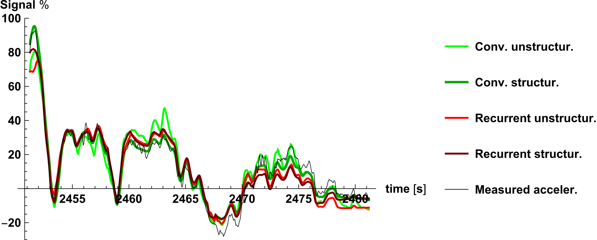
— Da Lio, M., Bortoluzzi, D. and Rosati Papini, G.P. "Modelling longitudinal vehicle dynamics with neural networks." Vehicle System Dynamics, 2019.
The plot shows the value of the accelleration over time for all types of networks.
The dark green line represents the fitting of the structured neural network that is the only network to estimate well the initial peak and the value around zero.
Physical inspiration for data driven approach
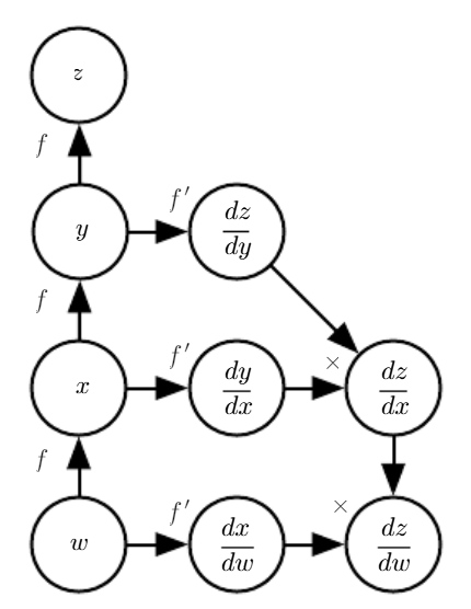
The model of the system is realized by neural network that is a:
- differentiable computational graph
- gradient descent algorithms are applicable
In this framework is simple to learn parameters of the model
In our case the characteristics are:
- this approach is flexible and modular
- the structure of the neural network takes inspiration from equations of motion
- the network is no black-box but it is explainable
- less parameters, less data for training, no overfitting, less experiments
— Goodfellow I., Bengio Y. and Courville A. Deep learning. 2015.
A neural network is a differentiable computational graph and in this framework gradient descent algorithms are applicable to easly tune the parameters.
This approach is flexible, it easy to add information to the model and what I don't know I can learn from data.
If I give a structure to the network that is inspired by the equation of motion, I reduce the number of the parameters and the needed data, therefore the experiments to collect it.
Moreover the network parameters are exaplainable.
But we can do more
It is possible to use neural network also for the control
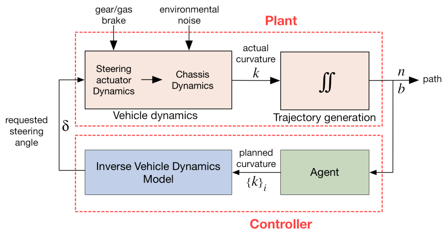
Use neural network for control
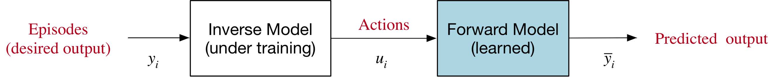
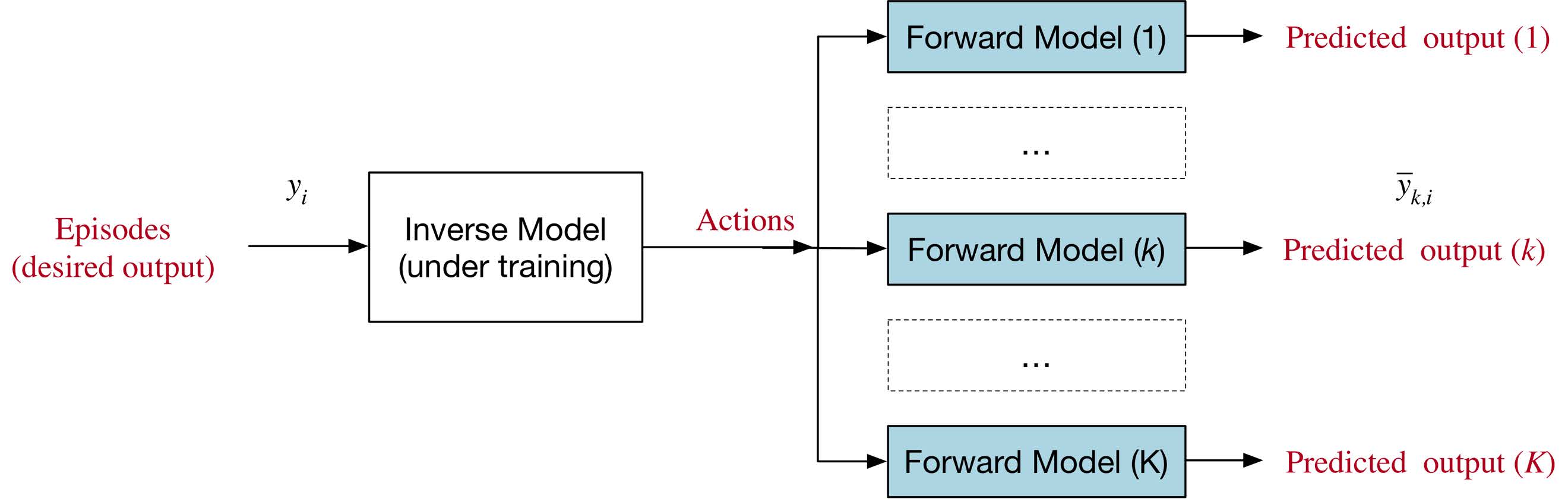
Synthesis of neural network for inverse modelling
using direct and inverse neural network in series (unsupervised method)
— Da Lio M., Donà R., Rosati Papini, G.P. et al. "A Mental Simulation Approach for Learning Neural-Network Predictive Control (in Self-Driving Cars)", IEEE Access, 2020.
Here is shown how to obtain neural network for control.
An interesting way is using the direct network already trained in series with a neural network that implement an inverse model.
In this way the input-output data of the series of the two networks has to be equal.
So we can expand the dataset by generating episodes at will for the training, reducing the number of experiments to collect them.
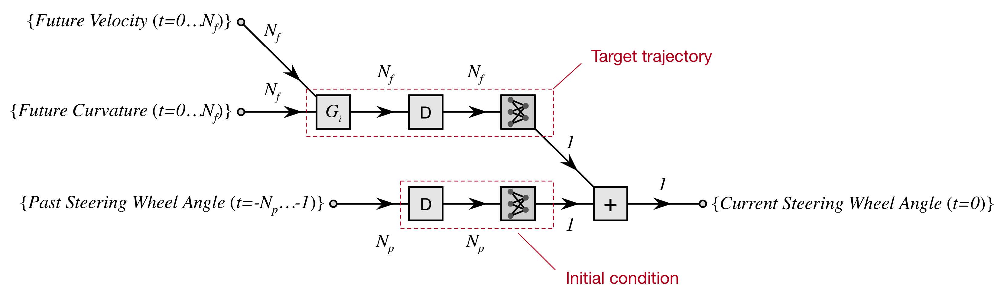
Here is shown an example of neural network for the inverse model of the Jeep Renegade lateral dynamics.
The four videos show how this architecture based on neural network inverse model works on different cars and simulators.
These results show the flexibility of this approach applied to different platforms.
On the left side there is the Jeep Renegade.
On the top the Miacar of DKFI.
On the bottom there are the two simulators: CarMaker and OpenDS.
Let's move on the second topic, deal with uncertain situation.
Think about this situation:
a pedestrian walks on the sidewalk and suddenly may cross the road.
It is pretty difficult to deal with this situation using a deterministic agent.
The agent predicts the behavior of the pedestrian only when he/she starts to cross the road, but it is too late.
The video show our agent before the integration of the neural network for safe speed.
The autonomous agent cannot stop in time due to high velocity.
I decided to deal with this situation using a reinforcement learning framework.
Let's see it in detail.
If this situation become a training scenario for a reinforcement learning framework I can deal with it.
This approach, however, has the problem of a long trainig phase, so in order to reduce it,
- we integrated our autonomous agant developed in dreams4cars with RL framework,
- so we focused on learning only what is fondamental, the safe speed. The neural network is not driving the car but is only gives a suggestion on the safe speed, in a way that, in case the pedestrian crosses the road the autonomous agent can stop the vehicle avoiding the impact.
- We used a simple neural network inside reinforcement learning framework so it can be explainable.
Neural Network for RL

The neural network chooses the requested cruising speed:
- the network possible actions are \(a=\{-\Delta_\text{RCS},0,\Delta_\text{RCS}\}\)
- the network estimates future reward for each possible actions:
- \(Q(s,a)\approx E\left[\sum_k^{\infty} \gamma^{k} r_{t+k}| s, a\right]\)
- a positive reward is given when the car reach without impact the end of the road
- during the simulation data are collected to train the network for a better estimation
The neural network does not drive the vehicle but suggests to the agent the safe speed by choosing the requested cruising speed.
The network gets in input the longitudinal and lateral position, velocity and curse of the pedestrian, the velocity of the car and the requested cruising speed.
The requested cruising speed is increased decreased or keeped by the network at each instant, as show in the picture.
In order to choose the correct safe speed during the training the network estimats the future reward for each action, at given a state, namely the Q value.
A positive reward is given to RL agent when the car reach without impact the end of the road, otherwise a negative reward.
During the simulation data are collected and the network is trained to a better estimates the action value Q.
Results - CRF Test of transfer learning
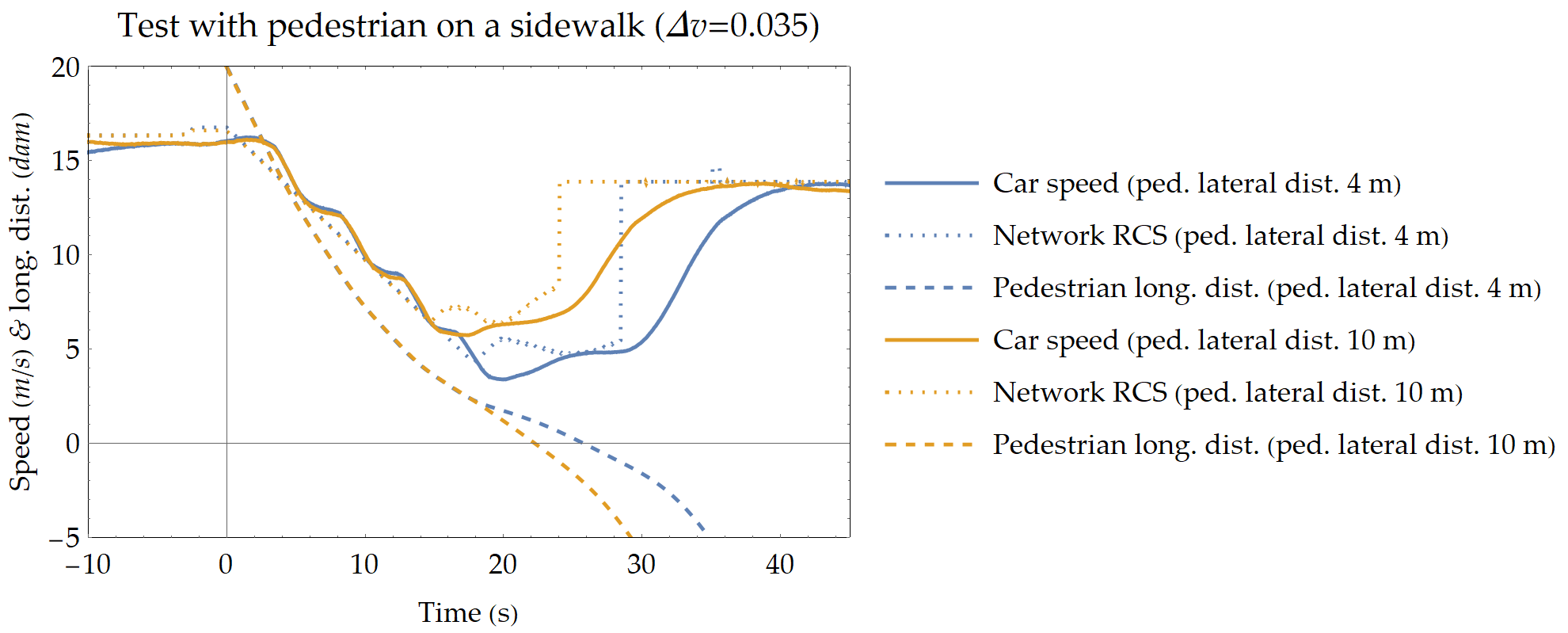
— Rosati Papini, G.P. et al. "A Reinforcement Learning Approach for Enacting Cautious Behaviours in Automated Driving Agents: Safe Speed Choice in the Interaction with Distracted Pedestrians.", IEEE Transactions on Intelligent Trasportation Systems, 2021.
This last slide show the results on the real CRF vehicle.
This result proves that it is possible to transfer what we learned in simulation to a real vehicle.
The network can be applied to a real vehicle because it does not drive the vehicle but only suggests the safe speed.
The blue lines are refered to the situation of 4 m of lateral distance of the pedestrian.
Whereas the orange lines are refered to the situation of 10 m.
The network is more cautious when the pedestrian is closer to the street.
Explainable RL approach on a focused issue

Deep Q-learning a reinforcement learning method
- temporal difference
- off policy
- value-based
- model-free
In our case the characteristics are:
- the network used is simple and therefore explainable
- use reinforcement learning only to learn what it is needed
- the network is integrated with an autonomous agent
- the transfer learning is applicable
- it is possible to synthesize a simple logic from the NN behavior
This tecnique is called deep q-learning and it is a temporal diference method, off policy, and model-free.
In our case the Q-learning is applied to a simple network so it can be exaplainable.
The RL is used only to learn what is needed, thanks to the integration with the autonomous agent.
The transfer learning is applicable.
Would also be possible to synthesize, as I did for the Poly-OWC, simple logic from the neural network behavior.
CACTO and CACTO-SL

Marge Trajectory Optimiazion with a Reinforcement Learning method and finally with Sobolev Learning
— Grandesso G., Alboni E. Rosati Papini, G.P. and et al. "CACTO: Continuous Actor-Critic With Trajectory Optimization—Towards Global Optimality" IEEE Robotic Automation Letter, 2023 — Alboni E. Grandesso G., Rosati Papini, G.P. and et al. "CACTO-SL: Using Sobolev Learning to improve Continuous Actor-Critic with Trajectory Optimization" Proceedings of Machine Learning Research, 2024.
Complex example of Model-Structured Neural Network
MSNN Longitudinal Estimator for ABS

MSNN for Lateral Vehicle Control


— Piccinini M., Zumerle M., Betz J. and Rosati Papini, G.P. "A Road Friction-Aware Anti-Lock Braking System Based on Model-Structured Neural Networks" IEEE Open Journal Intelligent Trasportation Systems, 2025 — Piccinini M., Mungiello A., Jank G. and Rosati Papini, G.P. and et al. "Model-Structured Neural Networks to Control the Steering Dynamics of Autonomous Race Cars" Proceedings of ITSC, 2025.
Some posters at the conferences


Robots - Quadruped
Collaboration: Prof. Andrea Del Prete
Go2 Robots

Challenges/Opportunities:
- Estimation of perturbation forces
- Managing contact forces
- Define the step orders
- Extension of the notion of motor cortex as way for motor control planning
- ...
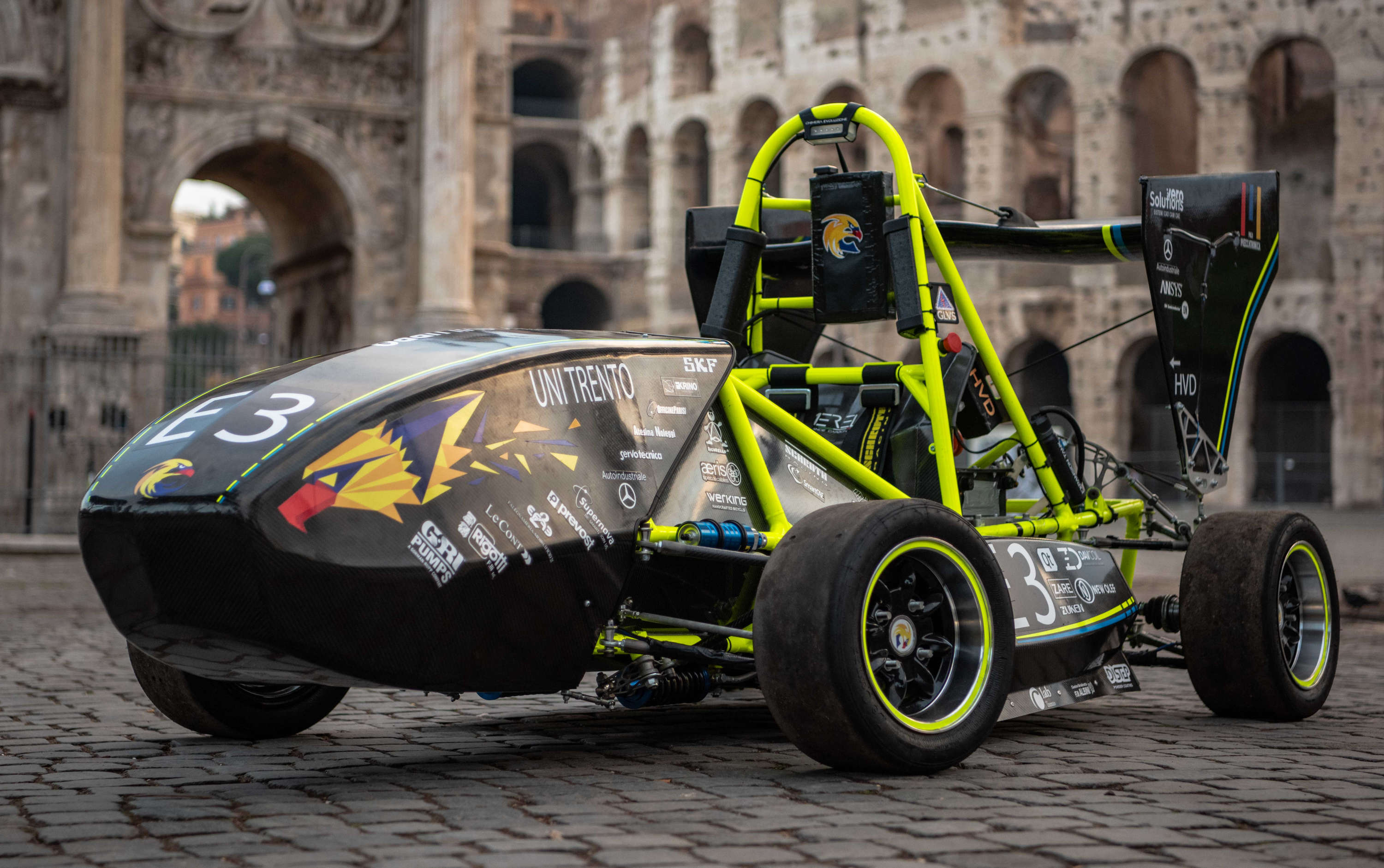
Vehicles - Full and Small Scale vehicles
Collaboration: Prof. Paolo Bosetti and Prof. Francesco Biral
SAE & F1tenth

Challenges/Opportunities:
- Integrate the autonomous angent with the driving system of the car
- Develop a inverse network for driving to the limits
- Test robust network in real application
- ...
Another field is vehicles, in particular set up a simulator and real vehicles.
Unmanned Aerial Vehicle
Collaboration: Prof. Davide Brunelli
QAV250 Holybro

Challenges/Opportunities:
- Control the system dynamics
- Estimation of air density
- Rapid path planning on embedded hardware
- ...